Predicting Heart Disease from the UCI Dataset

This project builds a model to predict the presence of heart disease. The UCI heart disease database carries 76 attributes, but all published experiments use a subset of 14. The target is an integer from 0 (no presence) to 4 — which, for simplicity, I reduce to binary classification: 0 versus 0 <.

The authors of the databases: Hungarian Institute of Cardiology, Budapest — Andras Janosi, M.D.; University Hospital, Zurich — William Steinbrunn, M.D.; University Hospital, Basel — Matthias Pfisterer, M.D.; V.A. Medical Center, Long Beach and Cleveland Clinic Foundation — Robert Detrano, M.D., Ph.D.

The attributes

	Description	Variable	Type
age	age in years	continuous	`int`
sex	1 = male, 0 = female	categorical	`int`
cp	chest pain type: 1 typical angina, 2 atypical angina, 3 non-anginal pain, 4 asymptomatic	categorical	`int`
trestbps	resting blood pressure in mm Hg	continuous	`float`
chol	serum cholesterol in mg/dl	continuous	`float`
fbs	fasting blood sugar > 120 mg/dl: 1 = true, 0 = false	categorical	`int`
restecg	0 normal, 1 ST-T wave abnormality, 2 left ventricular hypertrophy	categorical	`int`
thalach	maximum heart rate achieved	continuous	`float`
exang	exercise-induced angina (1 = yes, 0 = no)	categorical	`int`
oldpeak	ST depression induced by exercise relative to rest	continuous	`float`
slope	slope of the peak exercise ST segment: 1 upsloping, 2 flat, 3 downsloping	categorical	`int`
ca	number of major vessels (0–3) colored by fluoroscopy	continuous	`int`
thal	3 normal, 6 fixed defect, 7 reversible defect	categorical	`int`
target	diagnosis of heart disease (0 = false, 1 = true)	categorical	`int`

The flow: data fetching → wrangling → exploratory analysis → modeling → evaluation.

Imports

%matplotlib inline

import pandas as pd
import numpy as np
import matplotlib.pyplot as plt
import seaborn as sns
import statsmodels.api as sm
from sklearn.feature_selection import RFE
from sklearn import model_selection
from sklearn.model_selection import cross_val_score
from sklearn.model_selection import train_test_split as split
from sklearn.model_selection import GridSearchCV
from sklearn.linear_model import LogisticRegression
from sklearn import svm

sns.set(style="white")
sns.set(style="whitegrid", color_codes=True)

Data fetching

The UCI repository splits the data across four sites — Cleveland, Hungary, Switzerland, and Long Beach VA. I pull all four and concatenate them into a single frame.

link_cleveland = 'https://archive.ics.uci.edu/ml/machine-learning-databases/heart-disease/processed.cleveland.data'
link_hungarian = 'https://archive.ics.uci.edu/ml/machine-learning-databases/heart-disease/processed.hungarian.data'
link_swiss = 'https://archive.ics.uci.edu/ml/machine-learning-databases/heart-disease/processed.switzerland.data'
link_veniceb = 'https://archive.ics.uci.edu/ml/machine-learning-databases/heart-disease/processed.va.data'

links = [link_cleveland, link_hungarian, link_swiss, link_veniceb]
names = ['age', 'sex', 'cp', 'trestbps', 'chol', 'fbs', 'restecg', 'thalach', 'exang',
         'oldpeak', 'slope', 'ca', 'thal', 'target']

df = pd.concat(map(lambda x: pd.read_csv(x, names=names), links))
df.head()

Wrangling

Handling missing values

The datasets encode missing values as ?. Replacing them with NaN exposes how patchy some columns are — ca, thal, and slope are missing for the majority of rows.

df.replace('?', np.nan, inplace=True)
df.isnull().sum()

trestbps     59
chol         30
fbs          90
restecg       2
thalach      55
exang        55
oldpeak      62
slope       309
ca          611
thal        486

I drop the incomplete rows and reset the index. It costs a chunk of the data, but it leaves a clean, fully-populated frame to model on.

df.dropna(axis=0, inplace=True)
df.reset_index(drop=True, inplace=True)

Correcting data types

Everything arrives as strings. I coerce the categorical columns to int, the continuous ones to float, and collapse the target from {1,2,3,4} down to a single positive class.

df['ca'] = pd.to_numeric(df['ca'], errors='coerce')
df['thal'] = pd.to_numeric(df['thal'], errors='coerce')
df[['age', 'sex', 'cp', 'fbs', 'restecg', 'exang', 'ca', 'slope', 'thal']] = \
    df[['age', 'sex', 'cp', 'fbs', 'restecg', 'exang', 'ca', 'slope', 'thal']].astype(int)
df[['trestbps', 'chol', 'thalach', 'oldpeak']] = \
    df[['trestbps', 'chol', 'thalach', 'oldpeak']].astype(float)
df['target'].replace(to_replace=[1, 2, 3, 4], value=1, inplace=True)

Exploratory data analysis

Target

First, the class balance — is this a lopsided problem?

fig_target, ax = plt.subplots(nrows=1, ncols=1, figsize=(4, 4))
sns.countplot(x='target', data=df, ax=ax)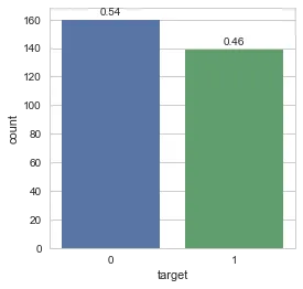

Target class balance — 54% no disease, 46% disease

Class balance of the target variable.

From the total dataset of 299 instances, 139 (46%) have a heart disease — close enough to balanced that accuracy is a reasonable headline metric.

Categorical features

For each categorical attribute I plot three views: the raw count, the count split by target, and the mean target (i.e. disease probability) per level.

def plotCategorial(attribute, labels, ax_index):
    sns.countplot(x=attribute, data=df, ax=axes[ax_index][0])
    sns.countplot(x='target', hue=attribute, data=df, ax=axes[ax_index][1])
    avg = df[[attribute, 'target']].groupby([attribute], as_index=False).mean()
    sns.barplot(x=attribute, y='target', hue=attribute, data=avg, ax=axes[ax_index][2])

    for t, l in zip(axes[ax_index][1].get_legend().texts, labels):
        t.set_text(l)
    for t, l in zip(axes[ax_index][2].get_legend().texts, labels):
        t.set_text(l)

categorial = [('sex', ['female', 'male']),
              ('cp', ['typical angina', 'atypical angina', 'non-anginal pain', 'asymptomatic']),
              ('fbs', ['fbs > 120mg', 'fbs < 120mg']),
              ('restecg', ['normal', 'ST-T wave', 'left ventricular']),
              ('exang', ['yes', 'no']),
              ('slope', ['upsloping', 'flat', 'downsloping']),
              ('thal', ['normal', 'fixed defect', 'reversible defect'])]

fig_categorial, axes = plt.subplots(nrows=len(categorial), ncols=3, figsize=(15, 30))
[plotCategorial(x[0], x[1], i) for i, x in enumerate(categorial)]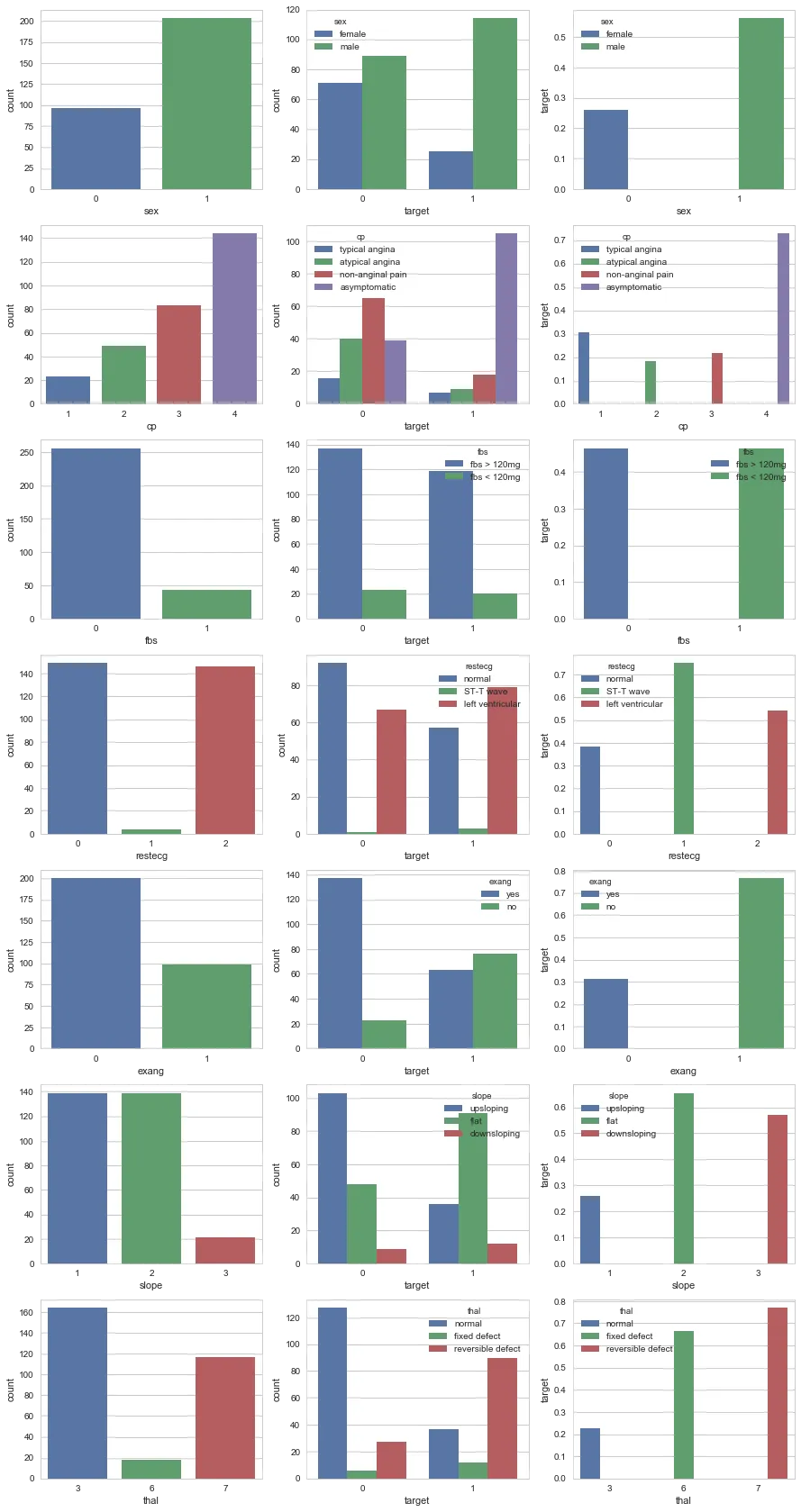

Categorical features — count, count-by-target, and disease probability per level

Each row: distribution, split by target, and mean disease probability per level.

Continuous features

For the continuous attributes I look at the distribution and a violin plot against the target.

def plotContinuous(attribute, xlabel, ax_index):
    sns.distplot(df[[attribute]], ax=axes[ax_index][0])
    axes[ax_index][0].set(xlabel=xlabel, ylabel='density')
    sns.violinplot(x='target', y=attribute, data=df, ax=axes[ax_index][1])

continuous = [('trestbps', 'blood pressure in mm Hg'),
              ('chol', 'serum cholestoral in mg/d'),
              ('thalach', 'maximum heart rate achieved'),
              ('oldpeak', 'ST depression by exercise relative to rest'),
              ('ca', '# major vessels: (0-3) colored by flourosopy')]

fig_continuous, axes = plt.subplots(nrows=len(continuous), ncols=2, figsize=(15, 22))
[plotContinuous(x[0], x[1], i) for i, x in enumerate(continuous)]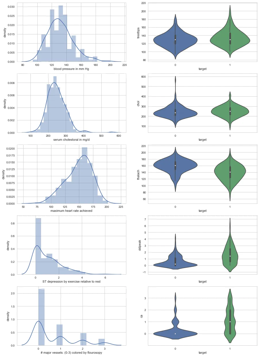

Continuous features — distribution and violin plot against the target

Each row: distribution and a violin plot split by target.

Age

fig_age, axes = plt.subplots(nrows=2, ncols=1, figsize=(15, 8))
facet_grid = sns.FacetGrid(df, hue='target')
facet_grid.map(sns.kdeplot, "age", shade=True, ax=axes[0])
legend_labels = ['disease false', 'disease true']
for t, l in zip(axes[0].get_legend().texts, legend_labels):
    t.set_text(l)
    axes[0].set(xlabel='age', ylabel='density')

avg = df[["age", "target"]].groupby(['age'], as_index=False).mean()
sns.barplot(x='age', y='target', data=avg, ax=axes[1])
axes[1].set(xlabel='age', ylabel='disease probability')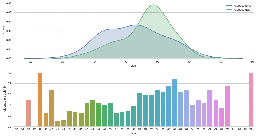

Age — density by target, and disease probability by age

Top: age density split by target. Bottom: disease probability by age.

Finalizing the data for modeling

Dummy variables

The multi-level categoricals (cp, restecg, slope, thal) get one-hot encoded so the linear models can use them.

cp_dummy = pd.get_dummies(df['cp'])
cp_dummy.rename(columns={1: 'cp_typical_angina', 2: 'cp_atypical_angina',
                         3: 'cp_non_angina', 4: 'cp_asymptomatic_angina'}, inplace=True)
restecg_dummy = pd.get_dummies(df['restecg'])
restecg_dummy.rename(columns={0: 'restecg_normal', 1: 'restecg_wave_abnorm',
                              2: 'restecg_ventricular_ht'}, inplace=True)
slope_dummy = pd.get_dummies(df['slope'])
slope_dummy.rename(columns={1: 'slope_upsloping', 2: 'slope_flat',
                            3: 'slope_downsloping'}, inplace=True)
thal_dummy = pd.get_dummies(df['thal'])
thal_dummy.rename(columns={3: 'thal_normal', 6: 'thal_fixed_defect',
                           7: 'thal_reversible_defect'}, inplace=True)
df = pd.concat([df, cp_dummy, restecg_dummy, slope_dummy, thal_dummy], axis=1)
df.drop(['cp', 'restecg', 'slope', 'thal'], axis=1, inplace=True)

Feature selection

Recursive Feature Elimination (RFE) selects features by recursively fitting the model and dropping the weakest, narrowing toward the subset that carries the signal.

df_X = df.drop('target', axis=1)
df_y = df['target']

rfe = RFE(LogisticRegression())
rfe.fit(df_X.values, df_y.values)
selected_features = [col for i, col in enumerate(df_X.columns.values) if rfe.support_[i]]

selected_X = df_X[selected_features]
selected_y = df_y

lm = sm.Logit(selected_y, selected_X)
result = lm.fit()
print result.summary()

selected_X_train, selected_X_test, selected_y_train, selected_y_test = \
    split(selected_X, selected_y, test_size=0.3, random_state=0)

Modeling

Logistic regression

lr = LogisticRegression()
lr.fit(selected_X_train, selected_y_train)
print 'Accuracy: %.3f' % lr.score(selected_X_test, selected_y_test)

Accuracy: 0.844

Support vector machine

A grid search tunes the kernel, C, and gamma over 5-fold CV before fitting the chosen model.

parameters = [{'kernel': ['rbf'], 'gamma': [1e-4, 1e-3, 0.01, 0.1, 0.2, 0.5],
               'C': [1, 10, 100]},
              {'kernel': ['linear'], 'C': [1, 10, 100]}]
grid = GridSearchCV(svm.SVC(decision_function_shape='ovr'), parameters, cv=5)
grid.fit(selected_X_train, selected_y_train)

svm_linear = svm.SVC(kernel='linear', C=10)
svm_linear.fit(selected_X_train, selected_y_train)
print 'Accuracy: %.3f' % svm_linear.score(selected_X_test, selected_y_test)

Accuracy: 0.822

Cross-validation

A single train/test split can flatter a model. Ten-fold cross-validation is the real test of whether these numbers hold.

kfold = model_selection.KFold(n_splits=10, random_state=7)
models = [('Linear regression', lr),
          ('Support vector machine', svm_linear)]

for model in models:
    results = model_selection.cross_val_score(
        model[1], selected_X_train, selected_y_train, cv=kfold, scoring='accuracy')
    print 'Cross validated', model[0], 'Accuracy: %.3f' % results.mean()

Cross validated Linear regression      Accuracy: 0.856
Cross validated Support vector machine Accuracy: 0.842

The complete notebook and data-prep script live in the project repository on GitHub.

The attributes#

Imports#

Data fetching#

Wrangling#

Handling missing values#

Correcting data types#

Exploratory data analysis#

Target#

Categorical features#

Continuous features#

Age#

Finalizing the data for modeling#

Dummy variables#

Feature selection#

Modeling#

Logistic regression#

Support vector machine#

Cross-validation#

Exit 0 Is Not Success for an Agent Job

Capacity Planning for Agents: Measure Yield, Not Tokens

Agent Memory Wants a Wiki, Not a Vector Store